class: center, middle, inverse, title-slide # Data and visualization ### Prof. Maria Tackett --- layout: true <div class="my-footer"> <span> <a href="http://datasciencebox.org" target="_blank">datasciencebox.org</a> </span> </div> --- class: middle, center ## [Click for PDF of slides](03-data-and-viz.pdf) --- class: center, middle # Exploratory data analysis --- ## What is EDA? - .vocab[Exploratory data analysis (EDA)] is an approach to analyzing data sets to summarize the main characteristics. <br> - Often, EDA is visual. That's what we're focusing on today. <br> - We can also calculate summary statistics and perform data wrangling/manipulation/transformation at (or before) this stage of the analysis. --- class: center, middle # Data visualization --- ## Data visualization > *"The simple graph has brought more information to the data analyst’s mind than any other device." — John Tukey* <br> - .vocab[Data visualization] is the creation and study of the visual representation of data. <br> - There are many tools for visualizing data (R is one of them), and many approaches/systems within R for making data visualizations - We'll use **`ggplot2`**. --- ## ggplot2 in tidyverse .pull-left[ <img src="img/03/ggplot2-part-of-tidyverse.png" width="70%" /> ] .pull-right[ - **ggplot2** is tidyverse's data visualization package - The `gg` in "ggplot2" stands for Grammar of Graphics - It is inspired by the book **Grammar of Graphics** by Leland Wilkinson* 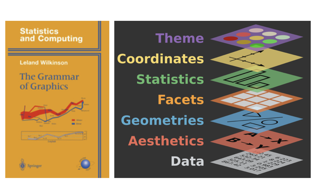 ] .footnote[ Source: [BloggoType](http://bloggotype.blogspot.com/2016/08/holiday-notes2-grammar-of-graphics.html) ] --- ## What is a Grammar of Graphics? A tool that allows for concisely describing the components of a graphic: <img src="img/03/grammar-of-graphics.png" width="70%" style="display: block; margin: auto;" /> --- ## What function is doing the plotting? ```r ggplot(data = starwars, mapping = aes(x = height, y = mass)) + * geom_point() + labs(title = "Mass vs. height of Starwars characters", x = "Height (cm)", y = "Weight (kg)") ``` ``` ## Warning: Removed 28 rows containing missing values (geom_point). ``` <img src="03-data-and-viz_files/figure-html/unnamed-chunk-4-1.png" style="display: block; margin: auto;" /> --- ## What is the dataset being plotted? ```r *ggplot(data = starwars, mapping = aes(x = height, y = mass)) + geom_point() + labs(title = "Mass vs. height of Starwars characters", x = "Height (cm)", y = "Weight (kg)") ``` ``` ## Warning: Removed 28 rows containing missing values (geom_point). ``` <img src="03-data-and-viz_files/figure-html/unnamed-chunk-5-1.png" style="display: block; margin: auto;" /> --- ## Which variable is on the x-axis? On the y-axis? ```r *ggplot(data = starwars, mapping = aes(x = height, y = mass)) + geom_point() + labs(title = "Mass vs. height of Starwars characters", x = "Height (cm)", y = "Weight (kg)") ``` ``` ## Warning: Removed 28 rows containing missing values (geom_point). ``` <img src="03-data-and-viz_files/figure-html/unnamed-chunk-6-1.png" style="display: block; margin: auto;" /> --- ## What does the warning mean? ```r ggplot(data = starwars, mapping = aes(x = height, y = mass)) + geom_point() + labs(title = "Mass vs. height of Starwars characters", x = "Height (cm)", y = "Weight (kg)") ``` ``` ## Warning: Removed 28 rows containing missing values (geom_point). ``` <img src="03-data-and-viz_files/figure-html/unnamed-chunk-7-1.png" style="display: block; margin: auto;" /> --- ## What does `geom_smooth()` do? ```r ggplot(data = starwars, mapping = aes(x = height, y = mass)) + geom_point() + * geom_smooth() + labs(title = "Mass vs. height of Starwars characters", x = "Height (cm)", y = "Weight (kg)") ``` <img src="03-data-and-viz_files/figure-html/unnamed-chunk-8-1.png" style="display: block; margin: auto;" /> --- ## Hello ggplot2! - `ggplot()` is the main function in ggplot2 and plots are constructed in layers - The structure of the code for plots can often be summarized as ```r ggplot + geom_xxx ``` <br> -- or, more precisely .small[ ```r ggplot(data = [dataset], mapping = aes(x = [x-variable], y = [y-variable])) + geom_xxx() + other options ``` ] --- ## Hello ggplot2! To use ggplot2 functions, first load tidyverse ```r library(tidyverse) ``` For help with the ggplot2, see [ggplot2.tidyverse.org](http://ggplot2.tidyverse.org/) --- class: center, middle # Visualizing Star Wars --- ## Dataset terminology .small[ ```r starwars ``` ``` ## # A tibble: 87 x 14 ## name height mass hair_color skin_color eye_color birth_year sex gender ## <chr> <int> <dbl> <chr> <chr> <chr> <dbl> <chr> <chr> ## 1 Luke… 172 77 other fair blue 19 male mascu… ## 2 C-3PO 167 75 none gold yellow 112 none mascu… ## 3 R2-D2 96 32 none white, bl… red 33 none mascu… ## 4 Dart… 202 136 none white yellow 41.9 male mascu… ## 5 Leia… 150 49 brown light brown 19 fema… femin… ## 6 Owen… 178 120 brown light blue 52 male mascu… ## 7 Beru… 165 75 brown light blue 47 fema… femin… ## 8 R5-D4 97 32 none white, red red NA none mascu… ## 9 Bigg… 183 84 black light brown 24 male mascu… ## 10 Obi-… 182 77 other fair blue-gray 57 male mascu… ## # … with 77 more rows, and 5 more variables: homeworld <chr>, species <chr>, ## # films <list>, vehicles <list>, starships <list> ``` ] Each row is an .vocab[observation]. Each column is a .vocab[variable] --- ## Luke Skywalker 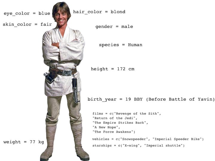 --- ## What's in the Star Wars data? Take a `glimpse` of the data: ```r glimpse(starwars) ``` ``` ## Rows: 87 ## Columns: 14 ## $ name <chr> "Luke Skywalker", "C-3PO", "R2-D2", "Darth Vader", "Leia O… ## $ height <int> 172, 167, 96, 202, 150, 178, 165, 97, 183, 182, 188, 180, … ## $ mass <dbl> 77.0, 75.0, 32.0, 136.0, 49.0, 120.0, 75.0, 32.0, 84.0, 77… ## $ hair_color <chr> "other", "none", "none", "none", "brown", "brown", "brown"… ## $ skin_color <chr> "fair", "gold", "white, blue", "white", "light", "light", … ## $ eye_color <chr> "blue", "yellow", "red", "yellow", "brown", "blue", "blue"… ## $ birth_year <dbl> 19.0, 112.0, 33.0, 41.9, 19.0, 52.0, 47.0, NA, 24.0, 57.0,… ## $ sex <chr> "male", "none", "none", "male", "female", "male", "female"… ## $ gender <chr> "masculine", "masculine", "masculine", "masculine", "femin… ## $ homeworld <chr> "Tatooine", "Tatooine", "Naboo", "Tatooine", "Alderaan", "… ## $ species <chr> "Human", "Droid", "Droid", "Human", "Human", "Human", "Hum… ## $ films <list> [<"The Empire Strikes Back", "Revenge of the Sith", "Retu… ## $ vehicles <list> [<"Snowspeeder", "Imperial Speeder Bike">, <>, <>, <>, "I… ## $ starships <list> [<"X-wing", "Imperial shuttle">, <>, <>, "TIE Advanced x1… ``` --- ## What's in the Star Wars data? Run the following **<u>in the Console</u>** to view the help ```r ?starwars ``` <img src="img/03/starwars-help.png" width="60%" /> --- ## Mass vs. height ```r ggplot(data = starwars, mapping = aes(x = height, y = mass)) + geom_point() ``` ``` ## Warning: Removed 28 rows containing missing values (geom_point). ``` <img src="03-data-and-viz_files/figure-html/unnamed-chunk-16-1.png" style="display: block; margin: auto;" /> --- ## What's that warning? - Not all characters have height and mass information (hence 28 of them not plotted) ``` ## Warning: Removed 28 rows containing missing values (geom_point). ``` - We can suppress warnings to save space on the output documents, but it's important to note them - To suppress warning: .center[ `{r code-chunk-label, warning=FALSE}` ] --- ## Mass vs. height .question[ How would you describe this **relationship**? Who is the not so tall but really heavy character? ] <img src="03-data-and-viz_files/figure-html/unnamed-chunk-17-1.png" style="display: block; margin: auto;" /> --- ## Jabba! <img src="img/03/jabbaplot.png" width="768" style="display: block; margin: auto;" /> --- ## Additional variables We can map additional variables to various features of the plot: - **aesthetics** - shape - color - size - alpha (transparency) - **faceting**: small multiples displaying different subsets --- class: center, middle # Aesthetics --- ## Aesthetics options Visual characteristics of plotting characters that can be **mapped to a specific variable** in the data are - `color` - `size` - `shape` - `alpha` (transparency) --- ## Mass vs. height + hair color ```r ggplot(data = starwars, mapping = aes(x = height, y = mass, color = hair_color)) + geom_point() ``` <img src="03-data-and-viz_files/figure-html/unnamed-chunk-19-1.png" style="display: block; margin: auto;" /> --- ## Mass vs. height + hair color Let's map `shape` and `color` to `hair_color` ```r ggplot(data = starwars, mapping = aes(x = height, y = mass, color = hair_color, * shape = hair_color )) + geom_point() ``` <img src="03-data-and-viz_files/figure-html/unnamed-chunk-20-1.png" style="display: block; margin: auto;" /> --- ### Mass vs. height + hair_color + birth year ```r ggplot(data = starwars, mapping = aes(x = height, y = mass, color = hair_color, shape = hair_color, * size = birth_year )) + geom_point() ``` <img src="03-data-and-viz_files/figure-html/plot-birth-year-1.png" style="display: block; margin: auto;" /> --- ## Mass vs. height + hair color Let's increase the size of all points across the board: ```r ggplot(data = starwars, mapping = aes(x = height, y = mass, color = hair_color)) + * geom_point(size = 3) ``` <img src="03-data-and-viz_files/figure-html/unnamed-chunk-21-1.png" style="display: block; margin: auto;" /> --- ## Aesthetics summary - Continuous variable are measured on a continuous scale - Discrete variables are measured (or often counted) on a discrete scale .small[ aesthetics | discrete | continuous ------------- | ------------------------ | ------------ color | rainbow of colors | gradient size | discrete steps | linear mapping between radius and value shape | different shape for each | shouldn't (and doesn't) work ] <br> .alert[Use aesthetics (`aes`) for mapping features of a plot to a variable, define the features in the `geom_xxx` for customization **<u>not</u>** mapped to a variable ] --- class: center, middle # Faceting --- ## Faceting options - Smaller plots that display different subsets of the data - Useful for exploring conditional relationships and large data ```r ggplot(data = starwars, mapping = aes(x = height, y = mass)) + * facet_grid(. ~ sex) + geom_point() + labs(title = "Mass vs. height of Starwars characters", * subtitle = "Faceted by sex", x = "Height (cm)", y = "Weight (kg)") ``` --- ```r ggplot(data = starwars, mapping = aes(x = height, y = mass)) + * facet_grid(. ~ sex) + geom_point() + labs(title = "Mass vs. height of Starwars characters", * subtitle = "Faceted by sex", x = "Height (cm)", y = "Weight (kg)") ``` <img src="03-data-and-viz_files/figure-html/unnamed-chunk-23-1.png" style="display: block; margin: auto;" /> --- ## Dive further... .question[ In the next few slides describe what each plot displays. Think about how the code relates to the output. ] -- <br><br><br> .alert[ The plots in the next few slides do not have proper titles, axis labels, etc, so you can more easily focus on what's happening in the plots. But you should always label your plots! ] --- ```r ggplot(data = starwars, mapping = aes(x = height, y = mass)) + geom_point() + facet_grid(hair_color ~ .) ``` <img src="03-data-and-viz_files/figure-html/unnamed-chunk-24-1.png" style="display: block; margin: auto;" /> --- ```r ggplot(data = starwars, mapping = aes(x = height, y = mass)) + geom_point() + facet_grid(. ~ hair_color) ``` <img src="03-data-and-viz_files/figure-html/unnamed-chunk-25-1.png" style="display: block; margin: auto;" /> --- ```r ggplot(data = starwars, mapping = aes(x = height, y = mass)) + geom_point() + facet_wrap(~ eye_color) ``` 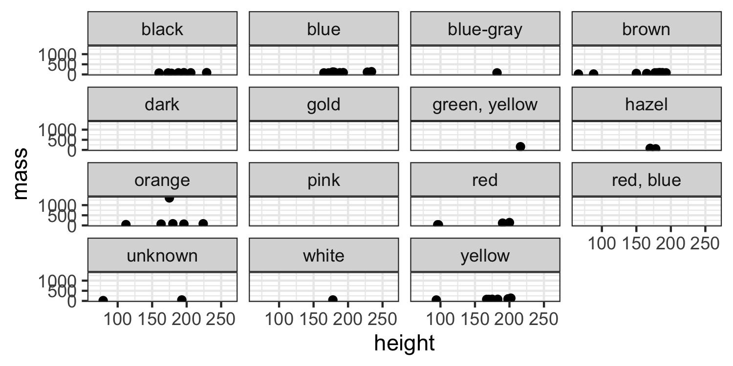<!-- --> --- ## Facet summary - `facet_grid()`: - 2d grid - `rows ~ cols` - use `.` for no split -- - `facet_wrap()`: 1d ribbon wrapped into 2d --- ## `ggplot2` supplementary resources 1. [ggplot2.tidyverse.org](https://ggplot2.tidyverse.org/) 2. `ggplot2` [cheat sheet](https://github.com/rstudio/cheatsheets/raw/master/data-visualization-2.1.pdf) 3. STA 523 `ggplot2` [slides](https://shawnsanto.com/files/sta523/slides/lec-3b-ggplot2.html#1) 4. [Top 50 `ggplot2` visualizations](http://r-statistics.co/Top50-Ggplot2-Visualizations-MasterList-R-Code.html) 5. [How the BBC uses `ggplot2`](https://medium.com/bbc-visual-and-data-journalism/how-the-bbc-visual-and-data-journalism-team-works-with-graphics-in-r-ed0b35693535) 6. [ggplot2: Elegant Graphics for Data Analysis](https://ggplot2-book.org/)