Web scrapingProf. Maria Tackett1

Click for PDF of slides

Scraping the web

Scraping the web: what? why?

Increasing amount of data is available on the web

Scraping the web: what? why?

Increasing amount of data is available on the web
These data are provided in an unstructured format: you can always copy&paste, but it's time-consuming and prone to errors

Scraping the web: what? why?

Increasing amount of data is available on the web
These data are provided in an unstructured format: you can always copy&paste, but it's time-consuming and prone to errors
Web scraping is the process of extracting this information automatically and transform it into a structured dataset

Scraping the web: what? why?

Increasing amount of data is available on the web
These data are provided in an unstructured format: you can always copy&paste, but it's time-consuming and prone to errors
Web scraping is the process of extracting this information automatically and transform it into a structured dataset
Two different scenarios:
- Screen scraping: extract data from source code of website, with html parser (easy) or regular expression matching (less easy).
- Web APIs (application programming interface): website offers a set of structured http requests that return JSON or XML files.

Web Scraping with rvest

Hypertext Markup Language (HTML)

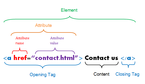
HTML describes the structure of a web page; your browser interprets the structure and contents and displays the results.
The basic building blocks include elements, tags, and attributes.
- an element is a component of an HTML document
- elements contain tags (start and end tag)
- attributes provide additional information about HTML elements

Hypertext Markup Language (HTML)

Simple HTML document

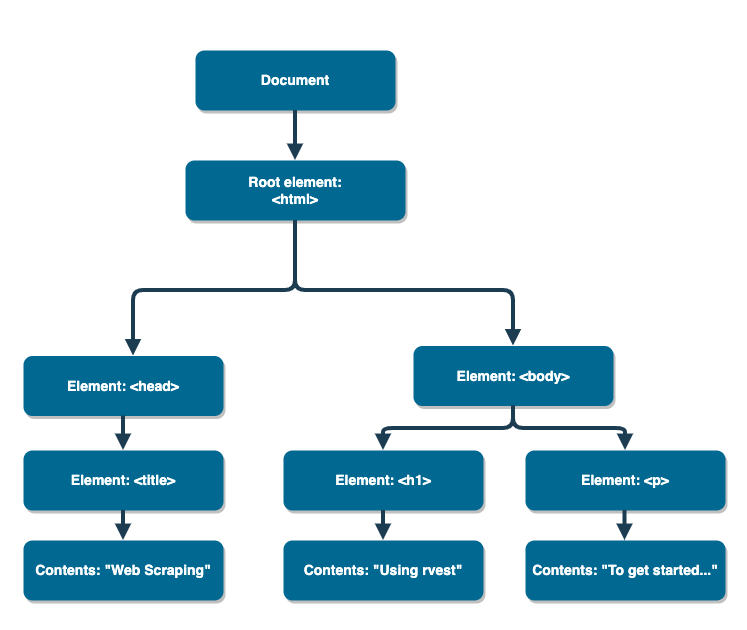
<html>
<head>
<title>Web Scraping</title>
</head>
<body>
<h1>Using rvest</h1>
<p>To get started...</p>
</body>
</html>

Simple HTML document

<html>
<head>
<title>Web Scraping</title>
</head>
<body>
<h1>Using rvest</h1>
<p>To get started...</p>
</body>
</html>

We can visualize this in a tree-like structure.

HTML tree-like structure

If we have access to an HTML document, then how can we easily extract information and get it in a format that's useful for analysis?

rvest

The rvest package makes basic processing and manipulation of HTML data straight forward
It's designed to work with pipelines built with %>%

Core rvest functions

read_html - Read HTML data from a url or character string
html_node - Select a specified node from HTML document
html_nodes - Select specified nodes from HTML document
html_table - Parse an HTML table into a data frame
html_text - Extract tag pairs' content
html_name - Extract tags' names
html_attrs - Extract all of each tag's attributes
html_attr - Extract tags' attribute value by name

Example: simple_html

Let's suppose we have the following HTML document from the example website with the URL simple_html

<html>
<head>
<title>Web Scraping</title>
</head>
<body>
<h1>Using rvest</h1>
<p>To get started...</p>
</body>
</html>

HTML in R

Read in the document with read_html().

page <- read_html(simple_html) #replace with URL in practice

HTML in R

Read in the document with read_html().

page <- read_html(simple_html) #replace with URL in practice

What does this look like?

HTML in R

Read in the document with read_html().

page <- read_html(simple_html) #replace with URL in practice

What does this look like?

page

## {html_document}
## <html>
## [1] <head>\n<meta http-equiv="Content-Type" content="text/html; charset=UTF-8 ...
## [2] <body>\n<h1>Using rvest</h1>\n<p>To get started...</p>\n</body>

Subset with `html_nodes()`

Let's extract the highlighted component below.

<html>
<head>
<title>Web Scraping</title>
</head>
<body>
<h1>Using rvest</h1>
<p>To get started...</p>
</body>
</html>

Subset with `html_nodes()`

Let's extract the highlighted component below.

<html>
<head>
<title>Web Scraping</title>
</head>
<body>
<h1>Using rvest</h1>
<p>To get started...</p>
</body>
</html>

h1_nodes <-page %>%
  html_nodes(css = "h1")
h1_nodes

## {xml_nodeset (1)}
## [1] <h1>Using rvest</h1>

Extract contents and tag name

Let's extract "Using rvest" and h1.

<html>
<head>
<title>Web Scraping</title>
</head>
<body>
<h1>Using rvest</h1>
<p>To get started...</p>
</body>
</html>

Extract contents and tag name

Let's extract "Using rvest" and h1.

<html>
<head>
<title>Web Scraping</title>
</head>
<body>
<h1>Using rvest</h1>
<p>To get started...</p>
</body>
</html>

h1_nodes %>% 
  html_text()

## [1] "Using rvest"

h1_nodes %>% 
  html_name()

## [1] "h1"

Scaling up

Most HTML documents are not as simple as what we just examined. There may be tables, hundreds of links, paragraphs of text, and more. Naturally, we may wonder:

How do we handle larger HTML documents?
How do we know what to provide to css in function html_nodes() when we attempt to subset the HTML document?
Are these functions in rvest vectorized? For instance, are we able to get all the content in the td tags on the slide that follows?

In Chrome, you can view the HTML document associated with a web page by going to View > Developer > View Source.

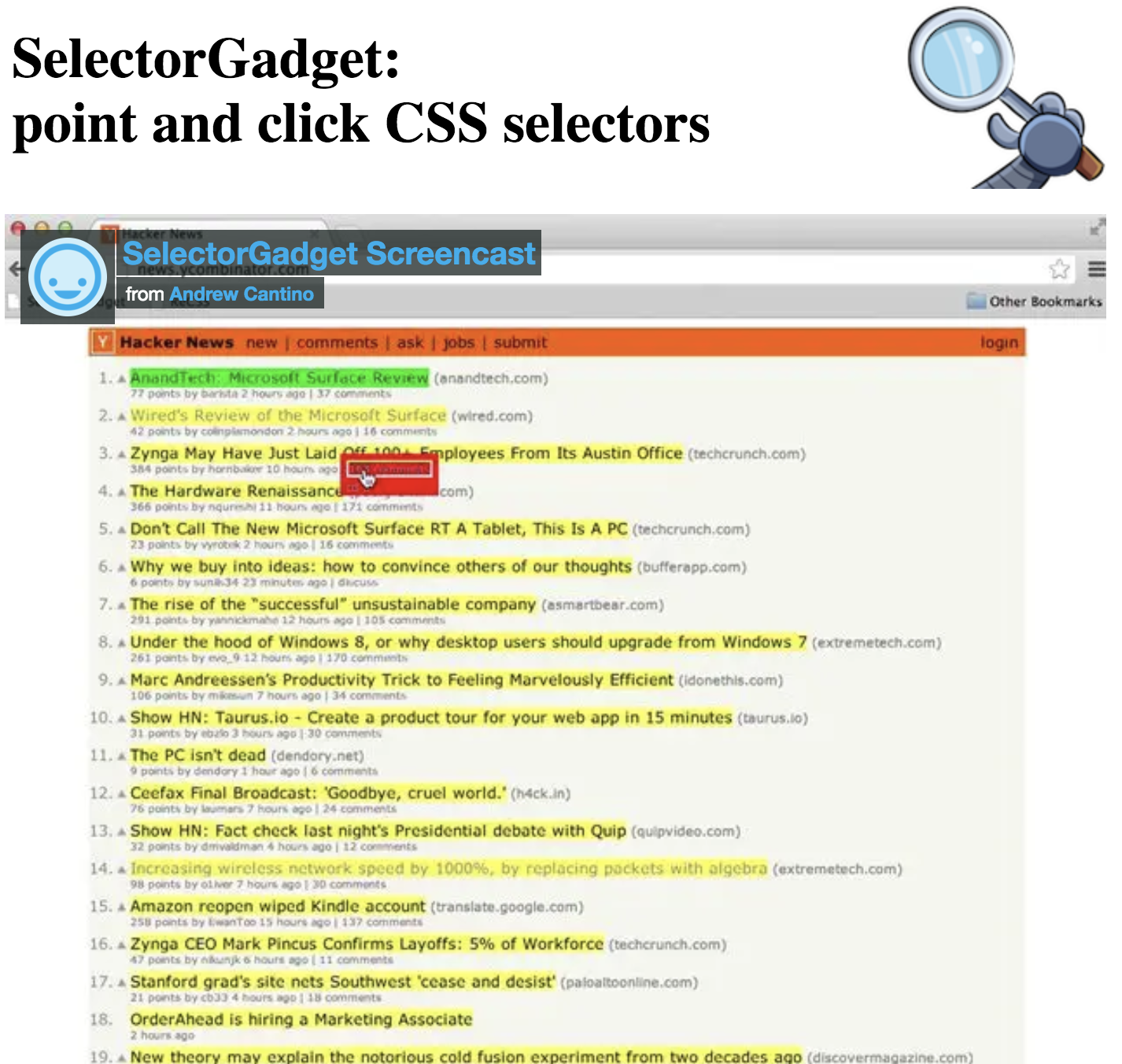
SelectorGadget

Open source tool that eases CSS selector generation and discovery
Can use through the Chrome Extension or the bookmark available on selectorgadget.com
Find out more on the SelectorGadget vignette

Using the SelectorGadget

Click on the app logo next to the search bar. A box will open in the bottom right of the website.
Click on a page element (it will turn green), SelectorGadget will generate a minimal CSS selector for that element, and will highlight (yellow) everything that is matched by the selector.

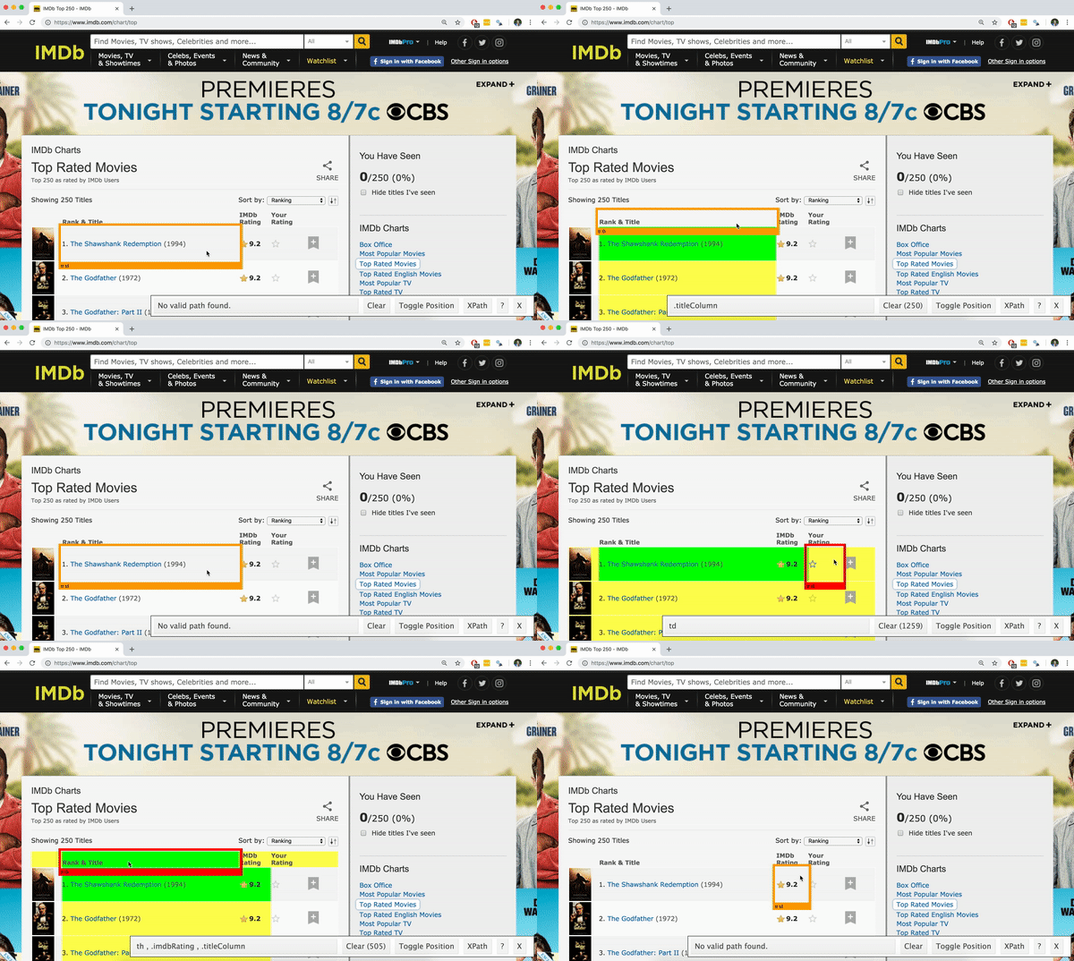
Click on a highlighted element to remove it from the selector (red), or click on an unhighlighted element to add it to the selector.
Through this process of selection and rejection, SelectorGadget helps you come up with the appropriate CSS selector for your needs.

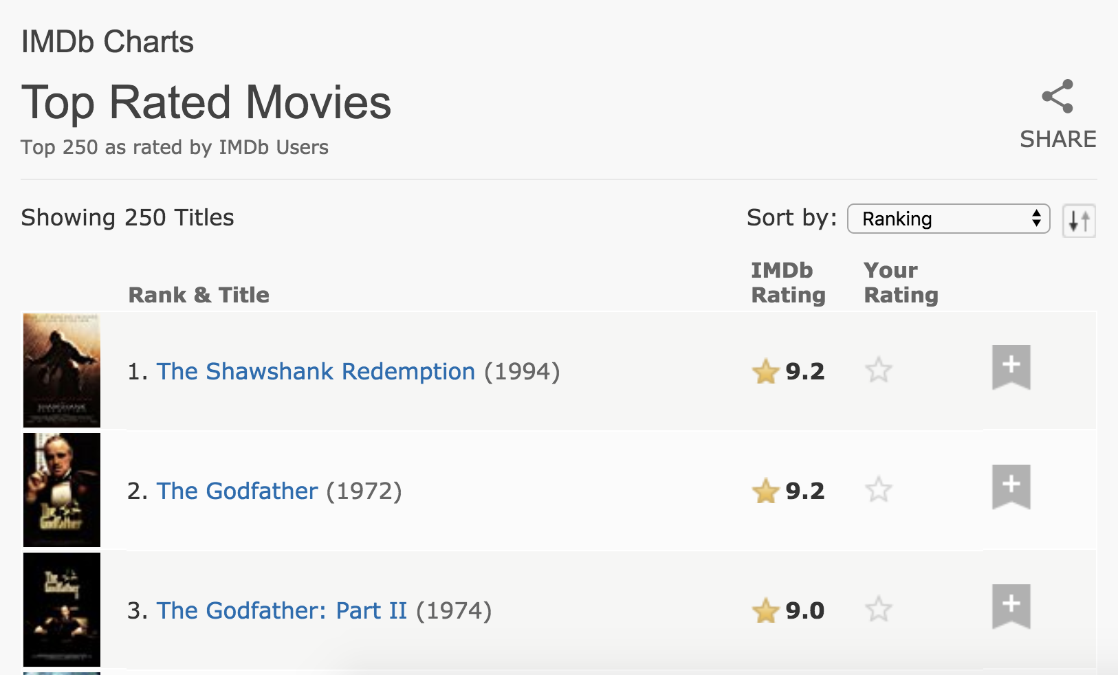
Top 250 movies on IMDB

Take a look at the source code, look for the table tag:
http://www.imdb.com/chart/top

First check if you're allowed!

library(robotstxt)
paths_allowed("http://www.imdb.com")

## [1] TRUE

vs. e.g.

paths_allowed("http://www.facebook.com")

## [1] FALSE

Select and format pieces

page <- read_html("http://www.imdb.com/chart/top")

Select and format pieces

page <- read_html("http://www.imdb.com/chart/top")

titles <- page %>%
  html_nodes(".titleColumn a") %>%
  html_text()

datasciencebox.org

Select and format piecespage <- read_html("http://www.imdb.com/chart/top")

titles <- page %>%
  html_nodes(".titleColumn a") %>%
  html_text()

years <- page %>%
  html_nodes(".secondaryInfo") %>%
  html_text() %>%
  str_replace("\\(", "") %>% # remove (
  str_replace("\\)", "") %>% # remove )
  as.numeric()

23

datasciencebox.org

Select and format piecespage <- read_html("http://www.imdb.com/chart/top")

titles <- page %>%
  html_nodes(".titleColumn a") %>%
  html_text()

years <- page %>%
  html_nodes(".secondaryInfo") %>%
  html_text() %>%
  str_replace("\\(", "") %>% # remove (
  str_replace("\\)", "") %>% # remove )
  as.numeric()

scores <- page %>%
  html_nodes("#main strong") %>%
  html_text() %>%
  as.numeric()

23

datasciencebox.org

Select and format piecespage <- read_html("http://www.imdb.com/chart/top")

titles <- page %>%
  html_nodes(".titleColumn a") %>%
  html_text()

years <- page %>%
  html_nodes(".secondaryInfo") %>%
  html_text() %>%
  str_replace("\\(", "") %>% # remove (
  str_replace("\\)", "") %>% # remove )
  as.numeric()

scores <- page %>%
  html_nodes("#main strong") %>%
  html_text() %>%
  as.numeric()

imdb_top_250 <- tibble(
  title = titles, year = years, score = scores)

23

imdb_top_250

## # A tibble: 250 x 3
##    title                                              year score
##    <chr>                                             <dbl> <dbl>
##  1 The Shawshank Redemption                           1994   9.2
##  2 The Godfather                                      1972   9.1
##  3 The Godfather: Part II                             1974   9  
##  4 The Dark Knight                                    2008   9  
##  5 12 Angry Men                                       1957   8.9
##  6 Schindler's List                                   1993   8.9
##  7 The Lord of the Rings: The Return of the King      2003   8.9
##  8 Pulp Fiction                                       1994   8.8
##  9 The Good, the Bad and the Ugly                     1966   8.8
## 10 The Lord of the Rings: The Fellowship of the Ring  2001   8.8
## # … with 240 more rows

imdb_top_250 %>%
  DT::datatable(options(list(dom = "p")))

Show entries

Search:

	title	year	score
1	The Shawshank Redemption	1994	9.2
2	The Godfather	1972	9.1
3	The Godfather: Part II	1974	9
4	The Dark Knight	2008	9
5	12 Angry Men	1957	8.9
6	Schindler's List	1993	8.9
7	The Lord of the Rings: The Return of the King	2003	8.9
8	Pulp Fiction	1994	8.8
9	The Good, the Bad and the Ugly	1966	8.8
10	The Lord of the Rings: The Fellowship of the Ring	2001	8.8

Showing 1 to 10 of 250 entries

Previous1 2 3 4 5…25Next

Clean up / enhance

May or may not be a lot of work depending on how messy the data are

See if you like what you got:

glimpse(imdb_top_250)

## Rows: 250
## Columns: 3
## $ title <chr> "The Shawshank Redemption", "The Godfather", "The Godfather: Pa…
## $ year  <dbl> 1994, 1972, 1974, 2008, 1957, 1993, 2003, 1994, 1966, 2001, 199…
## $ score <dbl> 9.2, 9.1, 9.0, 9.0, 8.9, 8.9, 8.9, 8.8, 8.8, 8.8, 8.8, 8.8, 8.7…

Clean up / enhance

May or may not be a lot of work depending on how messy the data are

See if you like what you got:

glimpse(imdb_top_250)

## Rows: 250
## Columns: 3
## $ title <chr> "The Shawshank Redemption", "The Godfather", "The Godfather: Pa…
## $ year  <dbl> 1994, 1972, 1974, 2008, 1957, 1993, 2003, 1994, 1966, 2001, 199…
## $ score <dbl> 9.2, 9.1, 9.0, 9.0, 8.9, 8.9, 8.9, 8.8, 8.8, 8.8, 8.8, 8.8, 8.7…

Add a variable for rank

imdb_top_250 <- imdb_top_250 %>%
  mutate(rank = 1:nrow(imdb_top_250))

imdb_top_250 %>%
  DT::datatable(options(list(dom = "p")), height = 350)

	title	year	score	rank
1	The Shawshank Redemption	1994	9.2	1
2	The Godfather	1972	9.1	2
3	The Godfather: Part II	1974	9	3
4	The Dark Knight	2008	9	4
5	12 Angry Men	1957	8.9	5
6	Schindler's List	1993	8.9	6
7	The Lord of the Rings: The Return of the King	2003	8.9	7
8	Pulp Fiction	1994	8.8	8
9	The Good, the Bad and the Ugly	1966	8.8	9
10	The Lord of the Rings: The Fellowship of the Ring	2001	8.8	10

Analyze

How would you go about answering this question: Which 1995 movies made the list?

Analyze

How would you go about answering this question: Which 1995 movies made the list?

imdb_top_250 %>% 
  filter(year == 1995)

## # A tibble: 8 x 4
##   title               year score  rank
##   <chr>              <dbl> <dbl> <int>
## 1 Se7en               1995   8.6    20
## 2 The Usual Suspects  1995   8.5    32
## 3 Braveheart          1995   8.3    78
## 4 Toy Story           1995   8.3    81
## 5 Heat                1995   8.2   123
## 6 Casino              1995   8.2   139
## 7 Before Sunrise      1995   8.1   191
## 8 La Haine            1995   8     228

Analyze

How would you go about answering this question: Which years have the most movies on the list?

Analyze

How would you go about answering this question: Which years have the most movies on the list?

imdb_top_250 %>% 
  group_by(year) %>%
  summarise(total = n()) %>%
  arrange(desc(total)) %>%
  head(5)

## # A tibble: 5 x 2
##    year total
##   <dbl> <int>
## 1  1995     8
## 2  2019     7
## 3  1957     6
## 4  2000     6
## 5  2004     6

How would you go about creating this visualization: Visualize the average yearly score for movies that made it on the top 250 list over time.

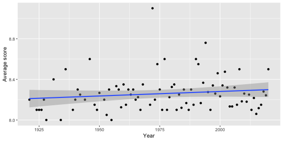
imdb_top_250 %>% 
  group_by(year) %>%
  summarise(avg_score = mean(score)) %>%
  ggplot(aes(y = avg_score, x = year)) +
    geom_point() +
    geom_smooth(method = "lm") +
    labs(x = "Year", y = "Average score")

Potential challenges

Unreliable formatting at the source
Data broken into many pages
...

Compare the display of information at raleigh.craigslist.org/search/apa to the list on the IMDB top 250 list. What challenges can you foresee in scraping a list of the available apartments?

↑, ←, Pg Up, k	Go to previous slide
↓, →, Pg Dn, Space, j	Go to next slide
Home	Go to first slide
End	Go to last slide
Number + Return	Go to specific slide
b / m / f	Toggle blackout / mirrored / fullscreen mode
c	Clone slideshow
p	Toggle presenter mode
t	Restart the presentation timer
?, h	Toggle this help

Web scraping

Prof. Maria Tackett

Click for PDF of slides

Scraping the web

Scraping the web: what? why?

Scraping the web: what? why?

Scraping the web: what? why?

Scraping the web: what? why?

Web Scraping with rvest

Hypertext Markup Language (HTML)

Hypertext Markup Language (HTML)

Simple HTML document

Simple HTML document

HTML tree-like structure

If we have access to an HTML document, then how can we easily extract information and get it in a format that's useful for analysis?

rvest

Core rvest functions

Example: simple_html

HTML in R

HTML in R

HTML in R

Subset with html_nodes()

Subset with html_nodes()

Extract contents and tag name

Extract contents and tag name

Scaling up

SelectorGadget

Using the SelectorGadget

Top 250 movies on IMDB

Top 250 movies on IMDB

First check if you're allowed!

Select and format pieces

Select and format pieces

Select and format pieces

Select and format pieces

Select and format pieces

Clean up / enhance

Clean up / enhance

Analyze

Analyze

Analyze

Analyze

Potential challenges

Click for PDF of slides

Help

Subset with `html_nodes()`

Subset with `html_nodes()`